Important Metrics for Test Methods:
Limits of Quantitation, Limits of Detection, Precision Error Profiles, Reportable Ranges

In immunoassay and bioassay tests, a regression curve describes the labeled response of standard calibrators at different concentrations of the reactive analyte.  Determining the range of concentrations that generate a meaningful response is of critical importance when developing a test method and evaluating assay results.  Whether developing an immunoassay test, a potency test, or a Tier III immunogenicity test, it is important to know what range of concentrations is bio-responsive under defined assay conditions.  This bio-responsive range is evaluated with respect to the requirements of the test.  Sometimes assay conditions need to be modified to shift the bio-responsive concentration range closer to a target range.  STATLIA MATRIX has many tools to aid these development efforts, and one of the most important tools is the determination of the precision error of concentrations in the regression curve.

Note about terminology.   Errors in concentration estimates are usually described in terms of accuracy and precision.  Accuracy, or bias, refers to how close the mean of concentration estimates approach the true concentration.  Precision is the amount of statistical variation around the concentration estimate, and this precision is usually expressed as %CV.  In STATLIA MATRIX, confidence limits are computed around the estimated concentration.  These confidence limits are expressed in concentration units and as a percentage of the estimated concentration.  This provides a clear measure for the analyst of the likely range that contains the true result.  To avoid confusion with established terminology, the confidence limit range around the concentration estimate is referred to as the precision error in STATLIA MATRIX and is expressed as a percentage of the estimated concentration or in concentration units.

Concentration Precision Error

Every concentration calculation from a regression curve is an estimation of the true concentration of that concentration estimate.  This means that there are confidence limits at a specified significance level around the estimate within which is the true concentration.  There are four physical factors that determine these confidence limits (the precision error) of a concentration estimate.  Each of these physical factors can be influenced by changes in the assay design, and these changes can thereby affect the precision error of the concentration estimates.

• Response variance. The response variance is the estimated variance at each concentration, obtained from a distribution of responses at specific concentrations (see Tech Note: Curve Weighting.) The smaller the estimated variance is at a concentration point, the lower the precision error is at that point.
• Response/concentration slope. The slope of a response/concentration point is the rate the regression is approaching the asymptotes at that point (see Tech Note: 5PL Curve Fitting). The steeper the slope is at a concentration point, the lower the precision error is at that point.
• Closeness of standard concentrations. Each standard concentration acts as an anchor point that constrains the shape of the regression in that region. The closer the closest standard concentration anchor points are to a point, the lower the precision error is at that point.
• Number of replicates. The more replicates there are for a concentration point, the lower the precision error is at that point.

Most attempts to derive the confidence interval around a concentration estimate use approaches such as the Wald method to linearize the regression around the curve parameters and linearize the confidence bounds of the concentration. While this approach is computationally easier, it works very poorly for ill-conditioned 4PL regressions and 5PL regressions. That is why these methods are not widely used. STATLIA MATRIX uses a modified Monte Carlo method to determine the variation in the fitted curve and the confidence interval around concentrations. This Monte Carlo method determines the confidence interval from a number of simulated fits using the same regression model that was used to fit the original data. Incorporated in these determinations are the response variance, the response/concentration slope, the closeness of adjacent standard points, and the number of replicates. An accurate estimation of the variation of the data is required to generate reliable simulations (see Tech Note: Curve Weighting). This Monte Carlo method accounts for the variation of the fitted curve and the variability of the unknown. The method works very well regardless whether the regression is well-conditioned or not, unlike methods that linearize the regression bounds. Because the same weighted regression model is used for the simulations, each fit fully accounts for the irregularities of any ill-conditioned regressions. The reliability of the confidence limit estimates increases with more simulations. Using this Monte Carlo method, the confidence interval of all concentrations for that response/concentration regression can be reliably determined, and a profile of concentration versus precision error can be generated for any specified significance level.

Using this Monte Carlo model profile, a lower limit of quantitation (LLOQ) and an upper limit of quantitation (ULOQ) can be determined for every regression curve at a user defined threshold of acceptable precision error. Further information on this Monte Carlo method can be found in the manuscript Determining the Error of Dose Estimates and Minimum and Maximum Acceptable Concentrations from Assays with Nonlinear Dose-Response Curves.

Precision Error Profiles and Limits of Quantitation (LOQs)

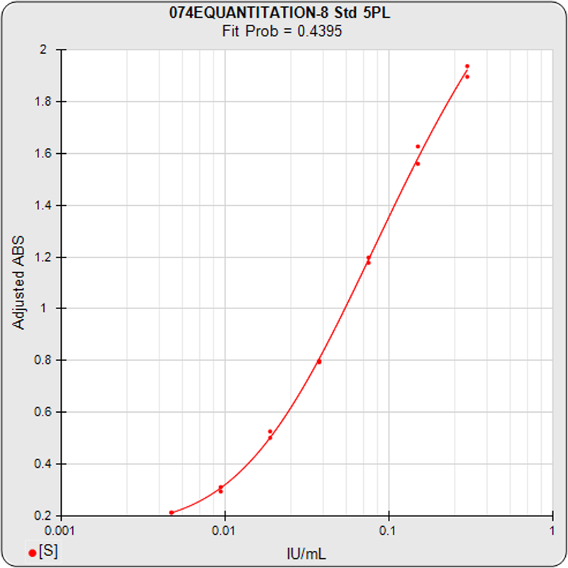
The standard curve describes the labeled response of standard calibrators at different concentrations of analyte. Concentration estimates from sample responses are made from this regression curve. Determining the precision error of each concentration estimate is an important step when evaluating the reliability of these results.

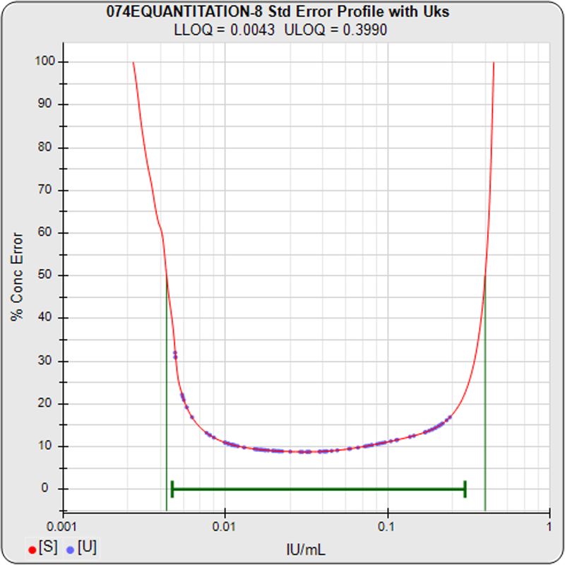
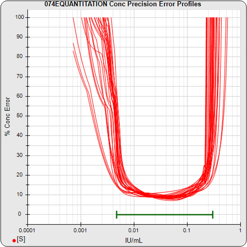
For the standard curve shown in the left graph, the precision error profile graph on the right plots the precision error of 100 concentration points (x-axis) of the standard curve linked together in red between a lower and upper threshold of 100% precision error (y-axis). These precision errors were computed using 12 Monte Carlo simulations at a confidence level of 0.95. Each concentration/precision error point factors in the response variance, the response/concentration slope, the closeness of adjacent standard points, and the number of replicates of the point.

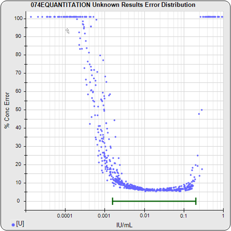
The precision error of each unknown specimen concentration, in blue, is computed in the same manner as the standard points. These unknown specimen points appear on the red standard curve profile plot if the unknown specimen has the same number of replicates as the standard dilutions. If the unknown specimen has fewer replicates than the standard dilutions, the blue point appears above the standard curve profile plot because that concentration estimate has more precision error. If the unknown specimen has more replicates than the standard dilutions, the blue point appears below the standard curve profile plot because that concentration estimate has less precision error. The unknown specimen point appears to the right of the red profile plot when its dilution factor is >1. Unknown specimens with precision errors greater than 100% are plotted immediately above 100% on the y-axis scale.

The lower and upper limits of quantitation (LLOQ, ULOQ) are determined for a user specified threshold of precision error (50% in the graph above) and are plotted as green vertical lines. The LLOQ and ULOQ values are listed in the subtitle at the top of the graph. The reportable range that was set by the user for the test method is plotted as a green horizontal line. Concentration results outside this reportable range are recorded in the database and in reports as less than or greater than the reportable range limit (immunoassay tests only). When evaluating the assay, the graph shows at a glance the targeted LOQs in relation to the reportable range for that assay, as well as the distribution of it’s unknown result precision errors.

Limits of Detection (LODs)

The limits of detection (LOD) are sometimes used as measure of the sensitivity of an assay system when reliable LLOQ and ULOQ measurements are not available. The lower limit of detection (LLOD) is the smallest concentration of analyte that can be statistically distinguished from the zero concentration but is too small to be quantified reliably. The LLOD is often determined using the upper confidence limit of a distribution of blank sample replicates having no analyte (sometimes called limit of blank or LOB). The weakness of this approach, of course, is that the LOB is only measuring the limits of analytical noise instead of the lowest amount of analyte that can be detected. Rarely used are designated LOD samples that contain analyte concentrations too low to quantify in the assay system that are statistically distinguishable from blank samples. The upper limit of detection (ULOD) is the largest concentration that can be statistically distinguished from an infinite, i.e. very large, concentration that is too large to be quantified reliably. The ULOD is seldom determined in practice.

STATLIA MATRIX computes an LLOD and ULOD from the standard curve itself, and the values obtained are actual limits of detection of the assay. Because they are not quantifiable like the limits of quantitation described above, the LODs only serve as an indicator of the sensitivity of the test method and should not be used in place of the actual quantitation limits.

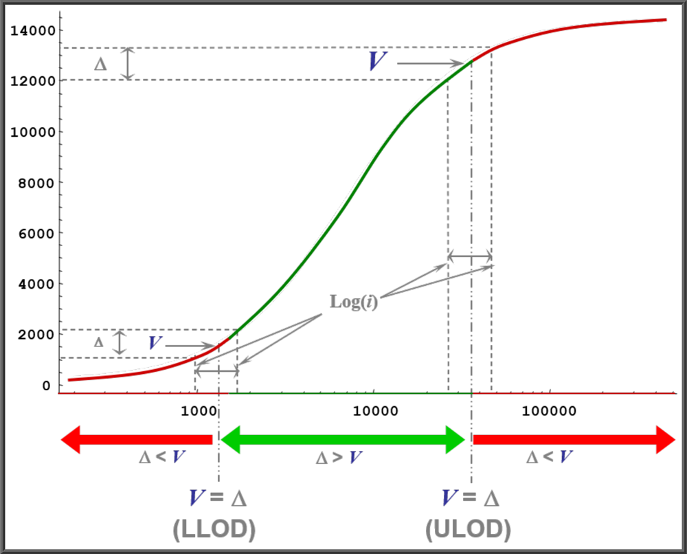
STATLIA MATRIX computes the LLOD and ULOD by modeling an empirical method to determine LLOD and ULOD of an assay system using a theoretical control sample with a continuous dilution series ranging from a very high concentration of analyte down to a very low concentration.  This is shown in the graph to the left (not drawn to scale).

• A dilution interval (“i” in graph) is set by the user. Log scaling is used to match the concentration x-axis scaling. The larger the dilution interval (i), the wider the LOD limits will be.
• This dilution interval (i) is advanced in continuous increments from the middle of the curve towards the low end of the curve to obtain the LLOD, then towards the high end of the curve to obtain the ULOD.
• The response difference (Δ) is computed for the concentrations at each end of the dilution interval (i) for each increment.
• The estimated variance (V) of the midpoint response of each increment is determined for the dilution interval (i). (An accurate estimation of the variance is required for accurate LLOD and ULOD determinations. See Tech Note: Curve Weighting).
• At each increment, a T test is performed to determine if the difference between Δ and V is significant at a user specified significance.
• The first dilution increment advancing in either direction whose Δ and V are not significantly different is then solved for the LLOD or ULOD concentration where Δ = V.

Establishing A Reportable Range From Pooled Assays

When developing a test method, it is very useful to examine the collective behavior of a pool of assays. This is done automatically in STATLIA MATRIX in the system Performance Analysis reports. A Performance Analysis is computed automatically after 6, 12, 20 and 30 assays have been completed. From these computations, the weighting regression, the QC metric ranges, and other performance metrics are saved. See Assay Development for more information about the extensive graphs and metrics produced. Among other important information, these graphs and metrics allow a reliable reportable range to be established for the test, one that includes the analytical measurement range (AMR) and the clinically reportable range (CRR).

Pooled Unknown Precision Errors

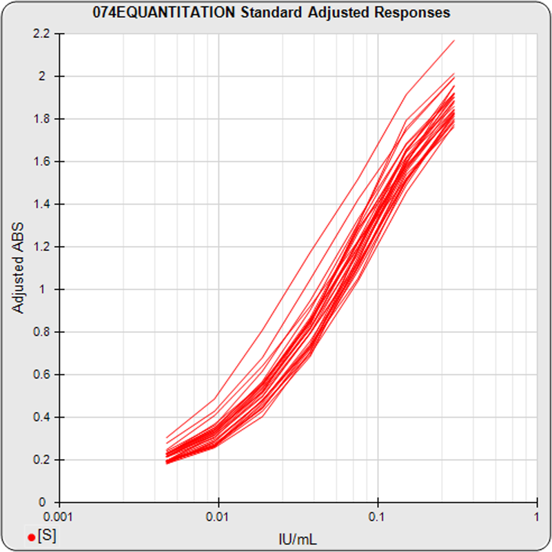
The graph on the left shows the standard dilution responses from a pool of 30 assays. The middle graph shows the precision error profiles from the standard curve regressions of these 30 assays. This middle graph shows the range of concentrations that are bio-responsive under the specific assay conditions implemented with this pool of assays. The horizontal green bar shows the user-defined reportable range set for these assays. The graph on the right shows the distribution of the precision errors of the unknown results from these pooled assays (immunoassay tests only). This graph shows how well the bio-responsive range, as well as the user-defined reportable range (green horizontal bar), matches the observed concentration range of the unknown population. The LLOQ, ULOQ, LLOD, and ULOD for each assay, and the statistics for their pooled metrics, are also computed. These metrics are valuable tools when comparing the performance of different protocol conditions or tests that have been transferred from one laboratory to another. The precision error profiles are also used to establish an effective dose range for a potency test. The bio-responsive range of the pooled tests should be evaluated with respect to the requirements of the test. If necessary, assay conditions can be modified to shift the bio-responsive concentration range closer to a target range. STATLIA MATRIX has many tools to aid these development efforts.

Finally, a Quality Assurance report is computed automatically every 30 new assays. This analysis performs the same computations as the Performance Analysis, and also performs a comparison of the behavior of these new assays to the behavior of the pooled 6, 12, 20, or 30 reference assays. This report alerts the laboratory to any behavioral changes that have occurred in the test method. A Quality Assurance analysis can also be computed comparing assays which utilized a specific reagent lot, or other criteria, to the reference assays.

REFERENCES

Bates DM, Watts DG.  Nonlinear Regression Analysis and Its Applications.  New York: Wiley, 1988.

Belanger BA, Davidian M, Giltinan DM  The Effect of Variance Function Estimation on Nonlinear Calibration Inference in Immunoassay Data.  Biometrics: 52, 158-175, 1996.

Boulanger B, Devanaryan V, Dewe W, Smith W.  Statistical Considerations in Analytical Method Validation.  Pharmaceutical Statistics Using SAS: A Practical Guide, 69-94, 2007 

Deming, SN.  The 4PL: A Guide to the use of the four-parameter logistic model in bioassay.  Statistical Designs, 2015.

DeSilva B, Smith W, Weiner R, Kelley M, Smolec J, Lee B, Khan M, Tacey R, Hill H, Celniker A.  Recommendations for the Bioanalytical Method Validation of Ligand-binding Assays to Support Pharmacokinetic Assessments of Macromolecules.  Pharmaceutical Research: 20 (11), 1885-1900, 2003.

Draper NR and Smith H.  Applied Regression Analysis, 3rd Edition. New York: Wiley, 1998.

Dudley RA, Edwards P, Ekins, RP, Finney, DJ, McKenzie, IGM, Raab, GM, Rodbard, D; Rodgers RPC.  Guidelines for Immunoassay Data Processing. Clinical Chemistry: 31 (8), 1264-1271, 1985. 

Dunn JR, Wild D.  Calibration Curve Fitting. The Immunoassay Handbook, Theory and Applications of Ligand Binding, ELISA and Related Techniques, 4th Edition, 323–336, 2013.

Gottschalk PG, Dunn JR. Determining the Error of Dose Estimates and Minimum and Maximum Acceptable Concentrations from Assays with Nonlinear Dose-Response Curves.  Computer Methods and Programs in Biomedicine, 204-215, 2005.

Gottschalk PG, Dunn JR. Measuring Parallelism, Linearity and Relative Potency in Immunoassay and Bioassay Data, Journal of Pharmaceutical Biostatistics 2005, 15 (3), 437–463.

Gottschalk PG, Dunn JR.  The Five Parameter Logistic: A Characterization And Comparison With The Four Parameter Logistic.  Analytical Biochemistry: 343, 54 – 65, 2005.

Karpinski, K. F.  Optimality Assessment in the Enzyme-Linked Immunosorbent Assay (ELIZA).  Biometrics 46, 381-390, 1990

Liu JS. Monte Carlo Strategies in Scientific Computing.  New York: Springer, 2004.

Press WH, Teukolsky SA, Vetterling WT, Flannery BP.  Numerical Recipes, 3rd Edition. New York: Cambridge University Press, 2007.

Seber GAF, Wild CJ.  Nonlinear Regression.  Hoboken NJ: Wiley, 2003.

www.brendan.com