There are 8 examples in this Tech Note that have been selected to show a range of curve shapes and calibrator dilution strategies computed with 4PL and 5PL curve models.   The effects of these different conditions on the assay results are shown in each example.  The assay curves are selected from ELISAs, ligand binding assays (LBA), and cell-based bioassays.  The 8 examples include:

• Weighting Versus No Weighting
• Curves Without A Plateau At One End
• Symmetric Curves
• Asymmetric Curves
• Extended Lower Plateau Curves With Additional Points
• Extended Upper And Lower Plateau Symmetric Curves
• Extended Lower Plateau Asymmetric Curves
• Extended Upper Plateau Asymmetric Curves

Four Parameter Logistic and Five Parameter Logistic Curve Fitting Models

Ligand binding assays (LBA) such as ELISAs and many cell-based bioassays require appropriate curve models to fit their nonlinear dose response data.  Dose response data points are the calibrator doses (e.g. ng/mL, IU/mL) versus their respective signal responses (e.g. OD, RLU).  The two most widely used curve models are the four parameter logistic (4PL) and the five parameter logistic (5PL) regressions.  Both the 4PL and 5PL are least squares regressions, meaning that a single formula is derived that provides the closest fit of all of the points to the curve model.  The 4PL curve model describes a sigmoidal shape that is symmetric around its inflection point (where the curve changes from convex to concave) in the middle of the curve.  The 5PL curve model describes a sigmoidal shape that is asymmetric with an inflection point above or below the middle of the curve.

For a linear regression, the coefficients of the line (Y = a + bX) are easily obtained from a simple algorithm.  For nonlinear models like the 4PL and 5PL, iterative numeric algorithms are used in a process called minimization to find the one curve that best fits the data out of the entire family of possible curves that the curve model can produce.   This is accomplished by adjusting the coefficients (parameters) of the curve model until the coefficients of the fitting equation result in the lowest possible RSSE (sum of squared residuals or residual sum of squares error).  A squared residual is the vertical distance between the observed point and the curve, squared, divided by the estimated variance at that point.  When weighted with accurately estimated variances of the normally distributed response data around each dose point, the curve with the lowest RSSE will be the Maximum Likelihood Estimate (MLE) of the true underlying regression curve as defined in regression statistics.  More about weighting and RSSE below.

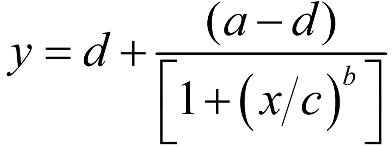
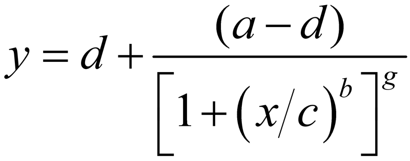
The equations for the 4PL and 5PL curve models are:

• Coefficients a and d control the location of the upper and the lower asymptotes of the equation. These are the values that the responses ( y ) approach as the log of the dose ( x ) approach 0 and infinity.
• Coefficient c controls the location of the transition on the dose ( x ) axis. This is the inflection point in the transition between the two asymptotes. In 4PL regressions, c is the midpoint between the two asymptotes.  In 5PL regressions, c is above or below the midpoint between the two asymptotes.
• Coefficient b is the slope at the transition point ( c ) and controls the rate of approach to the asymptotes. The sign of b controls whether the curve is monotonically ascending or descending.
• Coefficient g controls the asymmetry in a 5PL curve. This is the difference in the rates of approach from the inflection point ( c ) to the lower and the upper asymptotes. In a 4PL curve, g = 1 and is factored out.  In a 5PL curve, g is less than or greater than 1, depending upon the location of the inflection point.

For more information about the 4PL and 5PL models, see Tech Note: Computing Asymmetric Curves with 5PL and 4PL.

Weighting and Residuals

Statistical curve fitting uses a method called least squares regression fitting.  Least squares regression derives the one set of coefficients that has the smallest sum of squared residuals (RSSE) for that curve model.  As noted above, a squared residual is the vertical distance between the observed point and the curve, squared, divided by the estimated variance at that point. Weighting the squared residual errors with their estimated variances normalizes each point and allows all the points to contribute equally to the regression curve. 

The estimated variances are best obtained from a pooled distribution of responses at specific dose concentrations. Initial variance estimates can be made from the data of one assay, but more reliable variance estimates can be obtained from a pool of 6 or more historical assays. The estimated variances are derived from the calibrator response data from the pooled assays and fitted to a weighting equation.  The most common weighting equation model used is the formula AYB, where A is the error term, Y is the response, and B is the heteroscedastic change in the variances across the dose range.  The error term A can vary from 10-5 to 104 and the heteroscedascity term B can vary from 0.2 to 3 between different test methods and different label types.  With the fixed weighting equations 1/Y and 1/Y2 , A = 1 and B = 1 and 2, respectively.  F test goodness of fit probabilities average the replicate variances from the individual doses of that assay into a single estimated variance.  But it is common for the variances of points at the high-response end of a curve to be three or four orders of magnitude larger than variances of points at the low response end.  The greater the difference in magnitude between all the response points, the less applicable the single estimated variance used by the F test is to normalize the individual dose residuals.  Unweighted regressions use an estimated variance of 1 for all calibrator dilution points. 

The distribution of individual calibrator responses is approximately normal for most immunoassay and bioassay data.  The estimated variances used to compute the squared residual at each point are critical to obtaining the best curve fit.   This is because immunoassay and bioassay data are quite heteroscedastic (unequal variances) across their dose range, and it is important that each response is weighted by the inverse of the estimated variance of that response:

weight_i = 1/estimated variance_i

The reaction kinetics of the assay are a major factor in the heteroscedasticity of the response variances of each dose, and the reaction kinetics vary widely between different test methods.  Weighting the squared residual errors with the estimated variances at each point produce the most accurate concentration estimates.  Sample concentrations computed from unweighted curve fitting procedures can differ from properly weighted curves by hundreds of percent.

For more information about weighting, see Tech Note:  Curve Weighting.

Evaluating Curve Fits

According to regression statistics literature, the RSSE from an accurately weighted regression of normally distributed data will be chi square distributed with number of points minus number of parameter coefficients (N-P) degrees of freedom. This can be shown as follows:

The best fitting curve (MLE) is the curve that is the best estimate of the true underlying curve described by the dataset.  In statistics, one way to determine how well a curve is approaching the “true” curve is to determine how likely (probable) it is for the curve to have yielded the observed data under the assumption that the curve is actually the true curve.  The chi square probability (Fit Prob) is that likelihood, and it applies to any 5PL, 4PL or linear regression fit.  The Fit Prob is a statistical measure of how well a curve regression fits a set of data.  The Fit Prob applies equally well to fits of single logistic curves used in ELISA/LBA assays as well as to the unconstrained and constrained logistic curves used in potency assays (for more information, see Tech Note: Relative Potency and Parallelism in Potency Bioassays).   The number of data points (N) and parameter coefficients (P) determine the degrees of freedom (N-P), so the least parameterized model that has a similar or better RSSE than the other models will have the highest degrees of freedom and the best probability.

Since probabilities offer a familiar evaluation scale that is independent of the curve model or number of data points, the Fit Prob obtained from an accurately weighted least squares regression model is an ideal measure for goodness of fit.  A probability threshold for the Fit Prob (e.g. 0.05, 0.01) can be established for all test methods, regardless of number of points or parameters of each test curve.  And since the variability of the test method from the pooled assays is incorporated into the weighting, the Fit Prob is equally appropriate for well-behaved and ill-behaved test methods.  Because the RSSE is chi square distributed when the squared residuals are accurately weighted, the average RSSE from a pool of regression curves should approximately equal the degrees of freedom (N-P) and the average Fit Prob should be approximately 0.5.  This will confirm the reliability of the Fit Prob as a goodness of fit measure.  With appropriate weighting, the Fit Prob metric provides an effective goodness of fit metric, compared to the limitations of the F Test beyond a narrow range of responses having replicate variances of similar magnitude, and the lack of applicability of the R2 for nonlinear curves.

Weighting, Symmetric and Asymmetric Curve Shapes, and Calibrator Strategy Examples

The examples that follow in this Tech Note have been selected to show a range of curve shapes and calibrator dilution strategies.   The assay curves are selected from ELISAs, ligand binding assays (LBA), and cell-based bioassays having similar conditions.  Each assay example consist of three graphs and a metric table.

Standard Curve Graph
The graphs on the left show the 5PL or 4PL standard curve plot with the calibrator replicate points.  Note that in the standard curve graphs, scaling effects in semi-log standard curve graphs always make the low end appear to be a better fit than it actually is compared to the high end.

Squared Residuals Graph
The graphs in the middle show the squared residual errors (y-axis, red bars) between the observed and curve responses, squared, divided by the estimated variance for each calibrator point.  The response values are plotted on the linear x-axis. Squared residual values outside the graph limits are listed above their red bars. The squared residuals show the lack of fit of each calibrator dilution point.

%Bias Backfit Graphs
The graphs on the right show the %Bias backfit (y-axis, red bars) of the computed dose from the regression versus their actual calibrator dose ( ( ( computed – actual ) / actual ) x 100 ).  The calibrator points are plotted on the x-axis equidistant apart, not at dose level.   The QC limits for %Bias errors (red horizontal lines) in these graphs are set at +/-20%.   %Bias values outside the graph limits are listed above or below their red bars. The %Bias values show the likely error for results in that dose region based upon the backfit error of that calibrator dilution.

Curve Metrics Table
The 5PL and 4PL curve coefficients, degrees of freedom (N-P), RSSE, Fit Prob, and the weighting coefficients and weighting degrees of freedom are listed below each graph set.  All weighting estimates presented below (except the unweighted curve) were determined with the data from a pool of 6 assays of the same test method.  The differences between the error terms (Wt Coef A) in the 5PL and 4PL weighting equations are due to the residual (curve) error differences between the two curve models.  The heteroscedasticity (Wt Coef B) term is the same for both regression models.

Weighting Versus No Weighting

In the weighted regressions, the squared residuals of each response point are weighted by the estimated variances calculated from the weighting equation (AYB ) obtained from the pooled data of six assays.   The squared residuals of each calibrator in unweighted curves are divided by 1 (AYB : A=1, B=0) instead of an expected variance.  Unweighted regressions are predominantly fit to the high response points because those squared residuals, not normalized by their expected variances, can be three or four orders of magnitude larger than squared residuals of points at the low response end.  Determining the goodness of fit of an unweighted regression is more difficult than with a weighted regression.  F tests are used sometimes to assess curve fits, but this test is only effective within a narrow response range having replicate variances of similar magnitude.  This leaves few other options besides the R2 metric, with its lack of applicability to nonlinear curves, for evaluating an unweighted curve fit.

Weighted 5PL

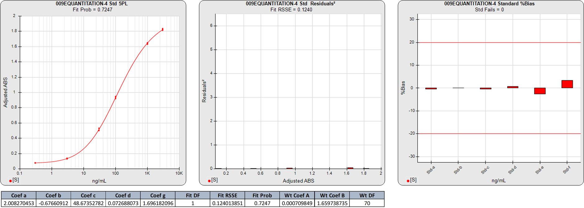
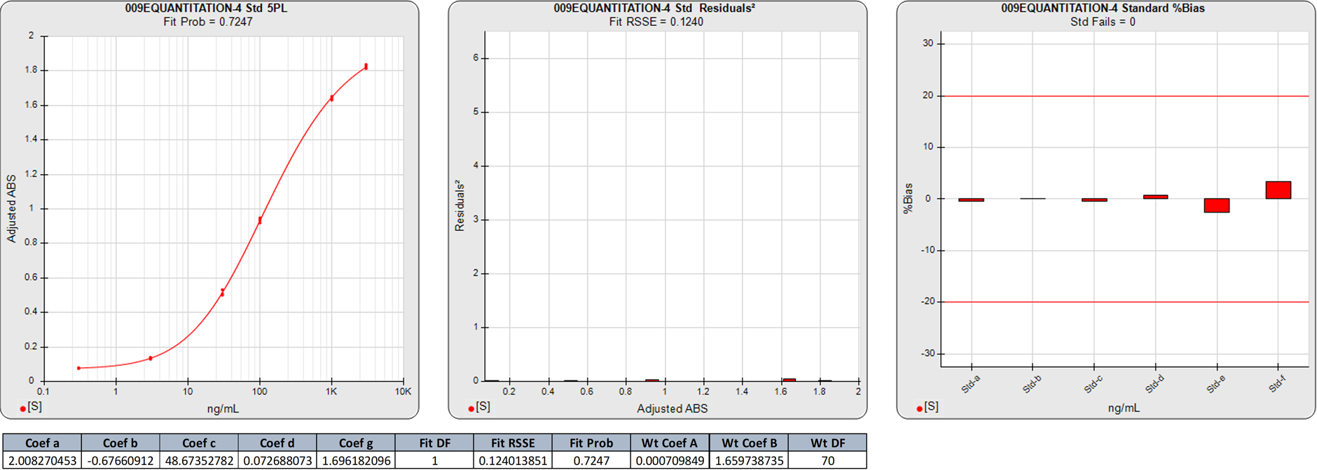
In this weighted 5PL regression of an ELISA curve, the weighting equation (AYB ) was determined from the pooled data of 6 assays (A=0.0007, B=1.6597).  There are 6 points on this 5PL curve, so the degrees of freedom (N-P) of the regression is 1. 

The 0.1240 RSSE is low (Fit Prob = 0.7247) indicating a good curve fit.  The %Bias backfit concentrations are close to their actual doses.

Unweighted 5PL

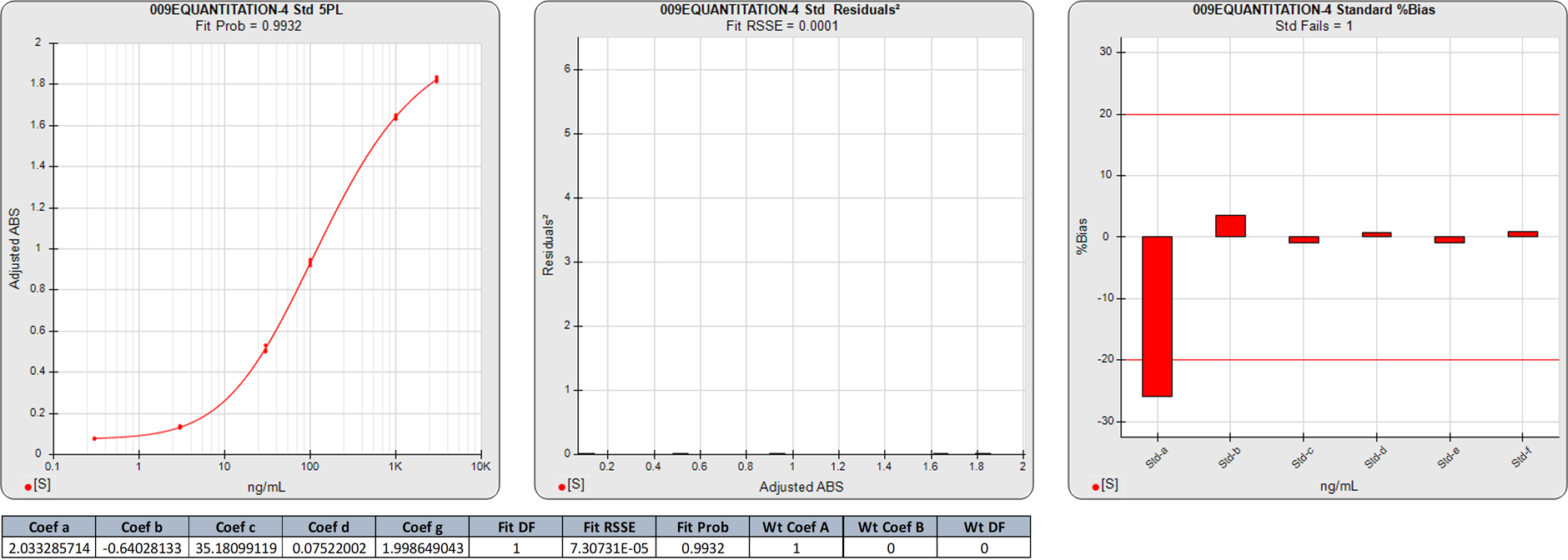
In this unweighted 5PL computation of the same ELISA curve as above, the substantial %Bias backfit error of the low calibrator is reflective of the small contribution of the low responses on the final regression solution.  The low %Bias at the high end is due to the greater dominance of the unweighted high responses in the regression fit.

The RSSE of unweighted regressions are not reflective of the relative (normalized) magnitude of the squared responses of the responses.  The Fit Prob is not a valid statistical value because the unweighted RSSE is not chi square distributed.

Note that this lack of fit in the unweighted 5PL is not obvious in the semi-log curve shown in the standard curve graph.

Curves Without A Plateau At One End

Curves that have only one defined sigmoidal end of the curve and do not reach an inflection point before the end calibrator point will have similar fits with 5PL and 4PL regressions.  The inflection point is where the curve changes from convex to concave.  Although the 4PL RSSE will usually be slightly larger than that of the 5PL, the extra degree of freedom (N-P) in the 4PL fit will give the 4PL least squares regression better averaging and often a slightly higher chi square probability (Fit Prob) than the 5PL regression when the degrees of freedom are low. 

In some extreme cases, the slope extends infinitely without ever reaching an inflection point.  Since the 4PL has the same shape at the lower convex end and the upper concave end, the fitting algorithms can derive an inflection point using the lower convex end shape for both the lower and upper end shapes.   But the 5PL defines a different shape for the lower convex end than for the upper concave end, so the fitting algorithms can’t use the shape of the lower end to help determine an inflection point.  In these cases, the upper asymptote approaches infinity and only the 4PL is practical.

Weighted 5PL

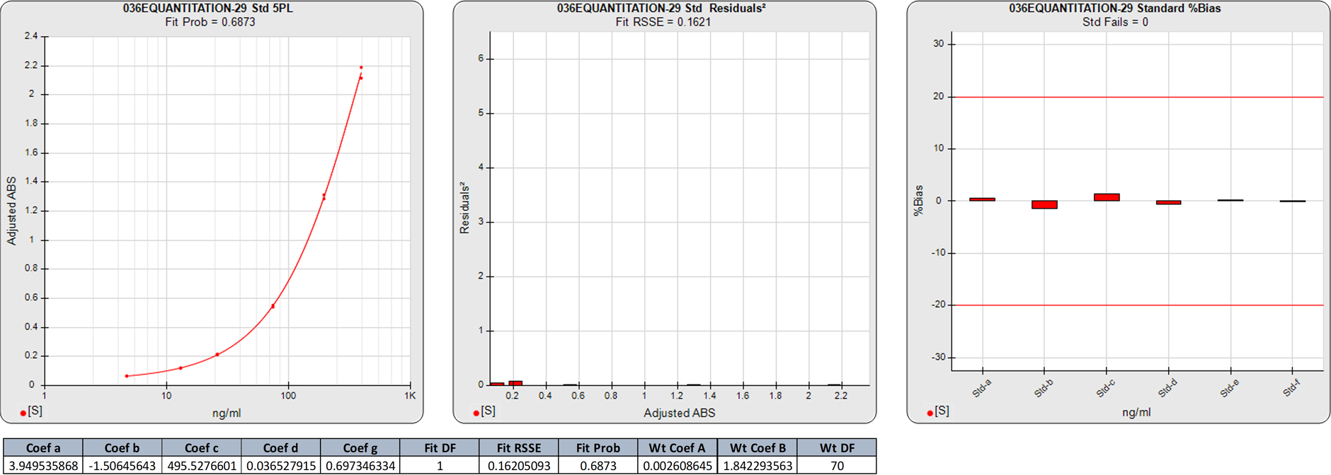
In this weighted 5PL regression of an ELISA curve, the estimated variances were calculated from the weighting equation obtained from the pooled data of 6 assays (A=0.0026, B=1.8423). There are 6 points on this 5PL curve, so the degrees of freedom (N-P) of the regression is 1.

The 0.1621 RSSE is low (Fit Prob = 0.6873) indicating a good curve fit.  The %Bias backfit concentrations are close to their actual doses.

Weighted 4PL

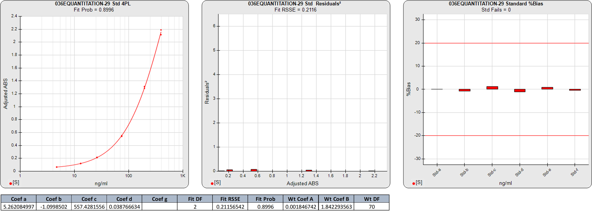
In this weighted 4PL regression of the same ELISA curve as above, the weighting equation was obtained from the pooled data of the same 6 assays (A=0.0018, B=1.8423).  There are 6 points on this 4PL curve, so the degrees of freedom (N-P) of the regression are 2.

The 0.2116 RSSE of this 4PL is a little higher than the 5PL RSSE, but the extra degree of freedom gives a higher Fit Prob (0.8996) than the 5PL.  The %Bias backfit concentrations are close to those from the 5PL, confirming the similarity of the two regression shapes. 

Because the calibrator points ended before an inflection point was reached, both the 5PL and 4PL curve shapes were very close, as shown by their similar RSSEs.

Symmetric Curves

Symmetric curves have similar (inverted) shapes at each end of the regression when the data points extend beyond the inflection point.  Like curves with only one plateau end region, these curves will have similar fits with 5PL and 4PL regressions.  Although the 4PL RSSE will usually be slightly larger than that of the 5PL, the extra degree of freedom (N-P) in the 4PL fit will give the 4PL least squares regression better averaging and often a higher Fit Prob than the 5PL regression when the degrees of freedom are low.

Weighted 5PL

In this weighted 5PL regression of an ELISA curve, the estimated variances were calculated from the weighting equation obtained from the pooled data of 6 assays (A=0.0026, B=1.8423). There are 6 points on this 5PL curve, so the degrees of freedom (N-P) of the regression is 1.

The 0.1621 RSSE is low (Fit Prob = 0.6873) indicating a good curve fit.  The %Bias backfit concentrations are close to their actual doses.

Weighted 4PL

In this weighted 4PL regression of the same ELISA curve as above, the weighting equation was obtained from the pooled data of the same 6 assays (A=0.0018, B=1.8423).  There are 6 points on this 4PL curve, so the degrees of freedom (N-P) of the regression are 2.

The 0.2116 RSSE of this 4PL is a little higher than the 5PL RSSE, but the extra degree of freedom gives a higher Fit Prob (0.8996) than the 5PL.  The %Bias backfit concentrations are close to those from the 5PL, confirming the similarity of the two regression shapes. 

Because the calibrator points ended before an inflection point was reached, both the 5PL and 4PL curve shapes were very close, as shown by their similar RSSEs.

Asymmetric Curves

Asymmetric curves have dissimilar (inverted) shapes at each end of the regression.  The 5PL can model these different shapes at each end of the curve, but the 4PL can only model the same (inverted) shape for both ends.  This means that, unlike relatively symmetric curves, there is a marked difference between the 5PL and 4PL regression fits.  This results in a significantly lower 5PL RSSE than that of the 4PL, and a higher Fit Prob for the 5PL than the 4PL despite the extra degree of freedom in the 4PL fit.  When the 4PL curve is weighted, the end shapes will be a single shape midway between the lower and upper shapes.  When the 4PL is unweighted, both ends are shaped close to the shape of the upper (high response) end.

Weighted 5PL

In this weighted 5PL regression of the first ELISA curve, there are 6 points on the 5PL curve, so the degrees of freedom (N-P) of this 5PL regression is 1.  The 0.1240 RSSE is low (Fit Prob = 0.7247) indicating a good curve fit.  The %Bias backfit concentrations are close to their actual doses.

Weighted 4PL

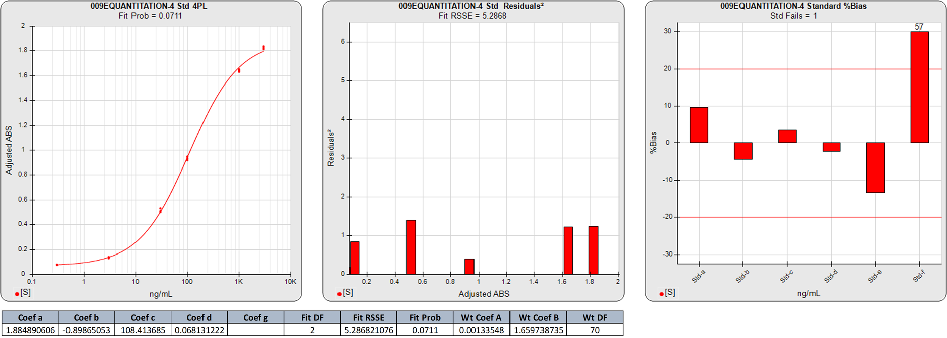
In this weighted 4PL regression of the same ELISA curve as above, the degrees of freedom (N-P) of this 4PL regression are 2.  The 5.2868 RSSE is a significantly higher than that of the 5PL, as illustrated by the higher individual squared residuals in the second graph.  The Fit Prob (0.0711) is much lower than that of the 5PL.  The %Bias backfit concentrations of the calibrators are considerably higher in the 4PL.

The significantly higher squared residuals in the 4PL confirm the asymmetry of the dose response data, and the higher %Bias values show the effect of this asymmetry on the 4PL results.  Note that this lack of fit in the 4PL is not obvious in the semi-log curve shown in the standard curve graph.

Extending Points into Plateau Regions

ELISA/LBA and bioassay regression curves are optimal when the response points of the standard calibrators are fairly equidistant from each other without any responses clustered or widely separated.  The more equidistant all of the calibrator responses are to each other, the lower the collective %Error and %Bias usually are throughout the dose range (for more information about %Error and determining LLOQ/ULOQ ranges see Tech Note: LOQs, LODs, Precision Error Profile, and Reportable Range). This gradient of responses can be an important factor when evaluating the quality (%Error, %Bias) of the regression results.  The gradient of calibrator concentrations is not a factor in the quality of the results.

Sometimes it is necessary to extend the limits of quantitation (LOQ) range in the test method.  Adding additional calibrator points to a plateau region can extend the LOQ range for that end region.  However, these extra points in the plateau region can result in an increase in the %Error and/or %Bias at the respective end of the curve, and sometimes throughout the entire dose range. Each plateaued response point cluster increases the influence of that region of the curve on the final regression curve, and these tightly grouped responses can sometimes be nonmonotonic.  Plateaued responses result in increased %Bias backfit values for those plateaued calibrators, and for the test sample results in that region.  This is because the response differences between the plateaued points are mostly random noise with little contribution from the reaction kinetics at those baseline or saturated analyte concentrations.

The assay curves that follow are selected from ELISAs, ligand binding assays (LBA), and cell-based bioassays having similar conditions.

Extended Lower Plateau Curves With Additional Points

Weighted 5PL

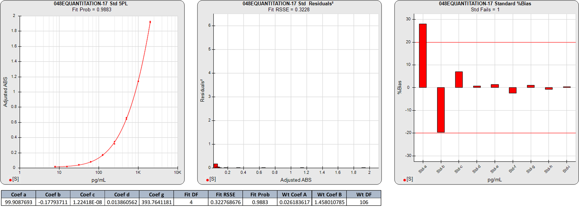
In this weighted 5PL regression of an ELISA curve, there are 9 points on the curve, so the degrees of freedom (N-P) are 4.   The calibrators assayed in this curve did not reach an inflection point.  The 0.3228 RSSE is very low (Fit Prob = 0.9883) indicating a very good curve fit for all of the calibrators. 

There is little difference in the responses of the lowest two points beyond noise even though the increase in concentration is double.  This has resulted in high %Bias backfit concentrations for those two doses regardless of the good curve fit.  Also, the responses of highest 3 doses are widely separated, so the regression shape is more influenced by the tighter spaced 6 points at the low end.

Weighted 4PL

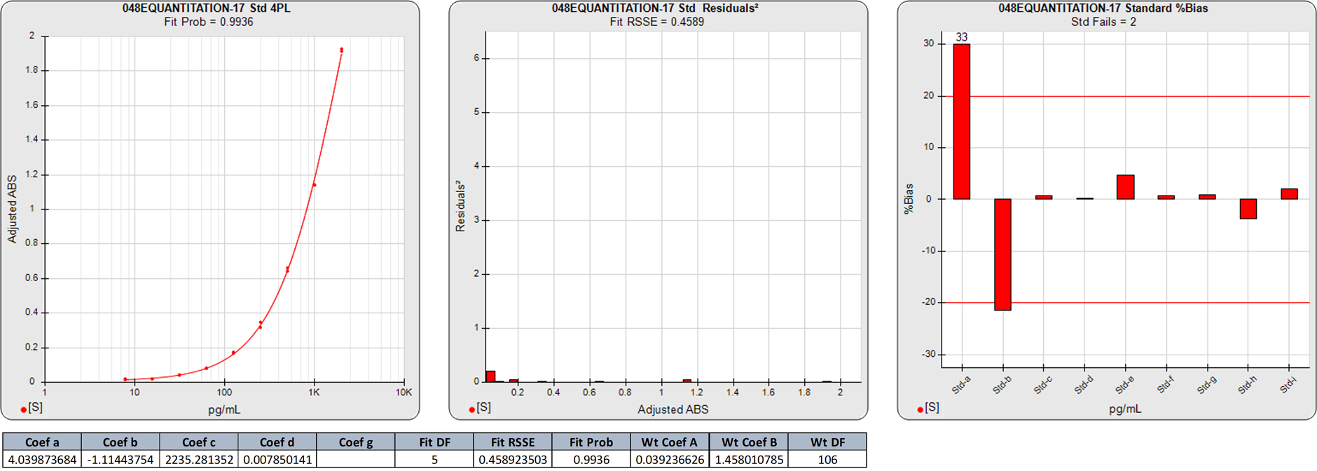
In this weighted 4PL regression of the same ELISA curve as above, the degrees of freedom (N-P) of the regression are 5.  The 0.4589 RSSE of this 4PL is a little higher than the 5PL RSSE, but the extra degree of freedom gives a slightly higher Fit Prob (0.9936) than the 5PL. 

Both the 5PL and 4PL curve shapes were very similar, as shown by their similar RSSEs and %Bias backfit concentrations.  Both models had large %Bias backfit for the two lowest doses, which had no material differences in response despite doubling the calibrator concentration.

Extended Upper and Lower Plateau Symmetric Curves

Weighted 5PL

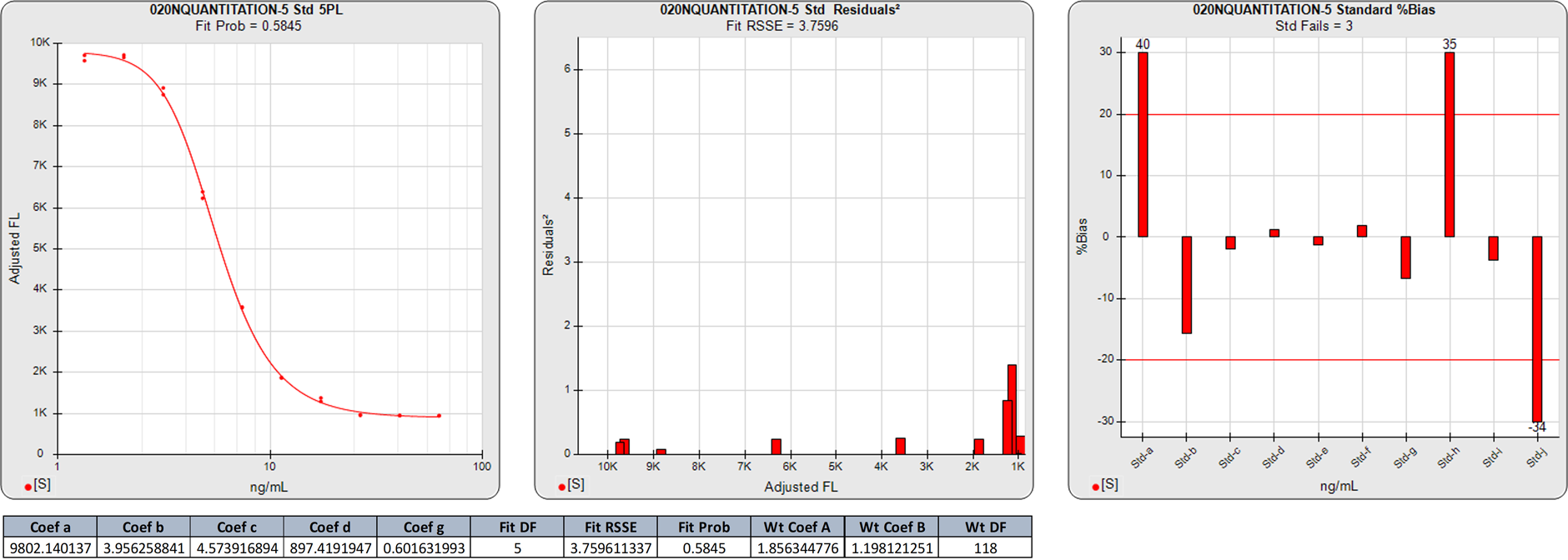
In this weighted 5PL regression of an LBA curve, there are 10 points on this 5PL curve, so the degrees of freedom (N-P) are 5.  The 3.7596 RSSE (Fit Prob = 0.5845) is a good curve fit. 

The two calibrator responses clustered at the high end and the three calibrator responses clustered at the low end in the middle squared residual graph are reflected in the high %Bias backfit concentrations for those doses regardless of the good curve fit.

Weighted 4PL

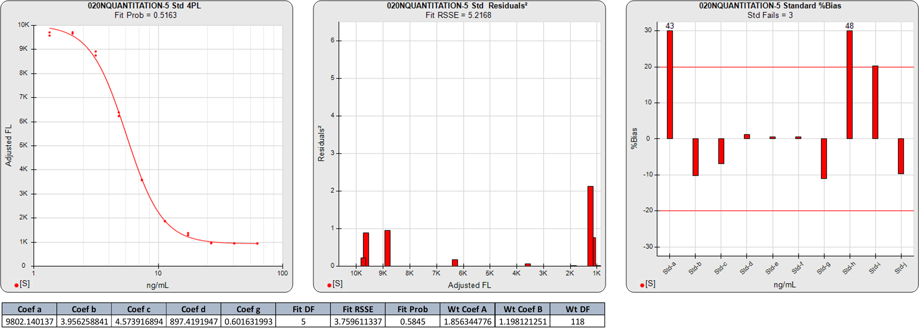
In this weighted 4PL regression of the same LBA curve as above, the degrees of freedom (N-P) of the regression are 6.  The 5.2168 RSSE of this 4PL yields a similar Fit Prob (0.5163) to the 5PL, confirming the similarity and symmetry of the two regression shapes. 

The large %Bias backfit of the plateaued high calibrator point and the three plateaued calibrator points at the low end are similar to those of the 5PL above.

Extended Lower Plateau Asymmetric Curves

Weighted 5PL

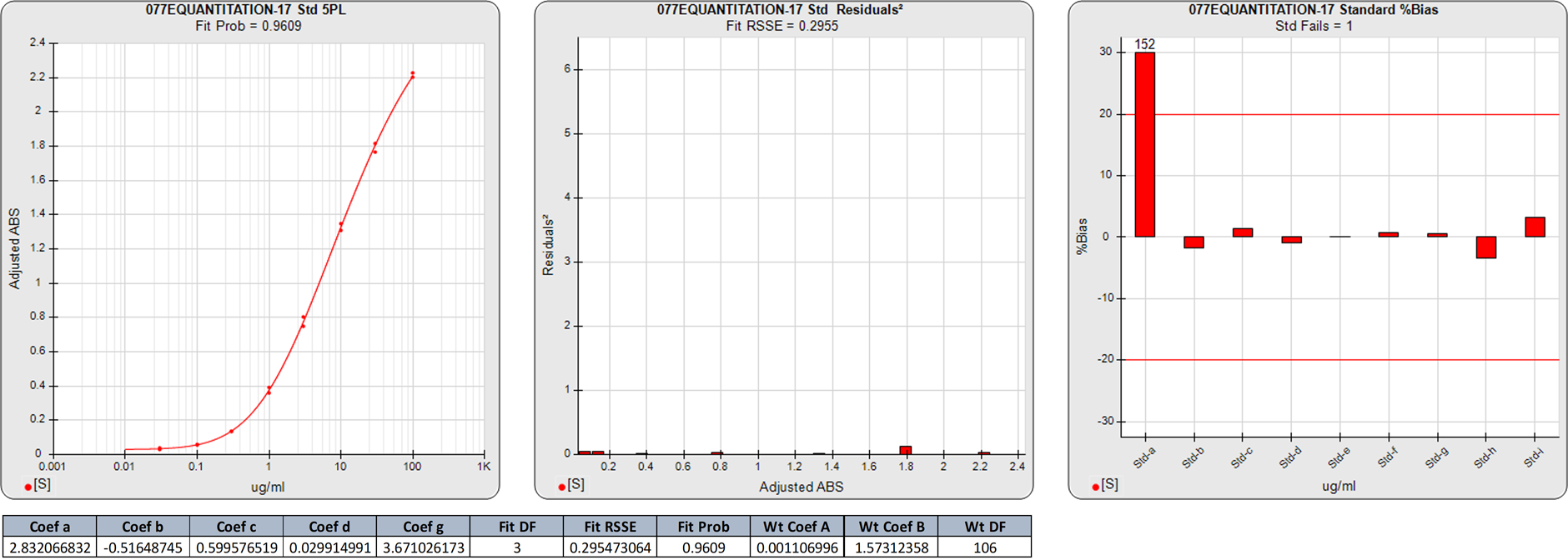
In this weighted 5PL regression of an ELISA curve, there are 9 points on the 5PL curve, so the degrees of freedom (N-P) are 4.  The 0.2955 RSSE (Fit Prob = 0.9609) is a very good curve fit. 

The two calibrator responses clustered at the low end of the curve are reflected in the high %Bias backfit concentrations for the lowest dose.  Although the lowest dose had a small squared residual, its response was essentially the same as the next dose despite having half the concentration of the higher point.

Weighted 4PL

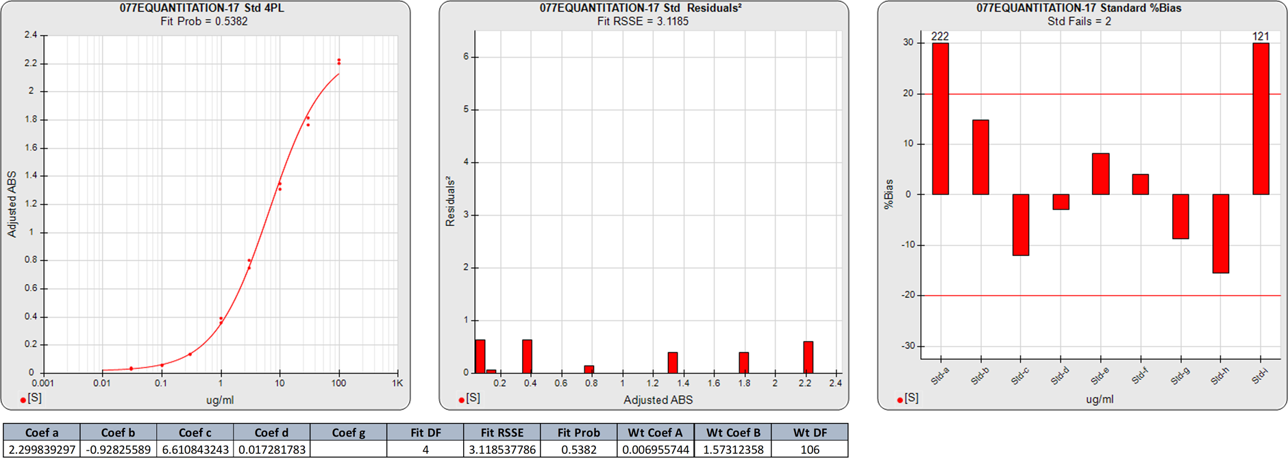
In this weighted 4PL regression of the same ELISA curve as above, the degrees of freedom (N-P) of the regression are 5.  The 3.1185 RSSE (Fit Prob = 0.5382) of this 4PL, while acceptable, is not as good as the 5PL fit, indicating the asymmetry of the curve. 

The plateaued low dose in the 4PL has the same high %Bias backfit as the 5PL produced.  But the substantially worse %Bias backfit concentrations for the remaining doses reflect the reduced ability of the 4PL to model the asymmetry of this curve.

Extended Upper Plateau Asymmetric Curves

Weighted 5PL

In this weighted 5PL regression of an ELISA curve, there are 9 points on the 5PL curve, so the degrees of freedom (N-P) are 4.  The 0.2955 RSSE (Fit Prob = 0.9609) is a very good curve fit. 

The two calibrator responses clustered at the low end of the curve are reflected in the high %Bias backfit concentrations for the lowest dose.  Although the lowest dose had a small squared residual, its response was essentially the same as the next dose despite having half the concentration of the higher point.

Weighted 4PL

In this weighted 4PL regression of the same cell-based bioassay curve as above, the asymmetry of the curve is apparent in the substantially poorer 4PL fit (RSSE = 8.6407, Fit Prob = 0.1948).  Since the 4PL regression is weighted, the lack of fit is balanced between the low convex end and high concave end of the curve, as is apparent in the squared residuals of the middle graph.  If the 4PL curve was unweighted, the lack of fit would be almost completely at the low end.

The very high %Bias backfit concentrations of the two highest doses observed in the 5PL fit are also present in the 4PL fit.  But the worse fit of the 4PL curve resulted in worse %Bias backfit concentrations for dose regions throughout the rest of the curve.

Choosing 4PL or 5PL and Calibrator Doses

The 4PL curve has been used extensively in immunoassay and bioassay data reduction.  The 4PL replaced logit and log transformations of these nonlinear responses which skew the results if the transformations are used beyond narrow ranges that are not typical for the dose response ranges of these assays.  When the immunoassay or bioassay curves are asymmetric, the 5PL curve has been shown to be the most effective curve model.  But the process of fitting the 5PL function is difficult for many data reduction software programs, with the result that the 4PL function has continued to be used even for highly asymmetric data. Even when the 5PL is offered, many software programs revert to a 4PL when they are unable to compute a 5PL fit.  However, advanced numerical algorithms plus accurate weighting estimates make it possible that even the most asymmetric and ill-behaved curve data can be computed with a 5PL regression.  Therefore, the decision for which fit model to use should depend upon which model is most appropriate for the data produced by the assays.

The 5PL requires at least 6 dose response calibrator points, whereas the 4PL only requires 5 calibrators.  If there are sufficient data points for both models, the most important metric to compare between the two models are how well each curve fit model fits the data.  The RSSE of the curve fits (when the regressions are appropriately weighted) can be expressed as a chi-square probability (Fit Prob).  Since the Fit Prob is determined from the RSSE and incorporates the number of points and number of parameters into this chi square probability, all curves are ranked using the same scale. And since the variability of the test method is incorporated into the weighting, the Fit Prob is equally appropriate for well-behaved and ill-behaved test methods. The Fit Prob is an effective metric for measuring and comparing the goodness of fit of regressions, compared to the F Test and the R2.   The F test is only effective within a narrow response range having replicate variances of similar magnitude, and the R2 has a lack of applicability to nonlinear curves.

A pool of assays can be collected and computed with both the 4PL and the 5PL.  The average Fit Prob of the assay curves between the two models will show whether the 4PL and 5PL models are similar or whether the curves are asymmetric, when the regressions are appropriately weighted.  The %Bias backfits of the individual calibrator points can also be compared between the two models.  If the data reduction software computes the %Error profile and LLOQ and ULOQ from the regression curve, the average %Error and the LOQ range obtained from the two models are also useful comparisons.  If the results are similar, either model is appropriate for that test method (the 4PL will compute faster and will have slightly better averaging of the regression points).  If the average Fit Prob from the 5PL is substantially better, the curve shapes are asymmetric and the 5PL should be used. 

The weighting equation used for weighting the 4PL or 5PL can be evaluated from the mean RSSE from the pooled curve fits.  If the weighting is appropriate, the average RSSE should approximately equal the degrees of freedom (N-P) of the regressions and the average Fit Prob should be approximately 0.5.  This will confirm the reliability of the Fit Prob as a goodness of fit measure. 

If the test method is still in the development phase, adding calibrators between widely separated calibrator response points can improve the quality of the results.  If a wider reportable range is necessary, extend the lower and/or upper plateau regions with additional calibrators.  Then recompute the 4PL or 5PL curves after masking the extended calibrator points one by one.  The calibrators can then be selected that yield the widest reportable range with acceptable %Bias backfits and, if available, %Errors.  This will allow a calibrator dose range to be chosen that will provide the best balance between optimal results and a sufficient reportable range.

REFERENCES

Bates DM, Watts DG.  Nonlinear Regression Analysis and Its Applications.  New York: Wiley, 1988.

Belanger BA, Davidian M, Giltinan DM The Effect of Variance Function Estimation on Nonlinear Calibration Inference in Immunoassay Data. Biometrics: 52, 158-175, 1996.

Boulanger B, Devanaryan V, Dewe W, Smith W. Statistical Considerations in Analytical Method Validation. Pharmaceutical Statistics Using SAS: A Practical Guide, 69-94, 2007.

Deming, SN.  The 4PL: A Guide to the use of the four-parameter logistic model in bioassay.  Statistical Designs, 2015.

DeSilva B, Smith W, Weiner R, Kelley M, Smolec J, Lee B, Khan M, Tacey R, Hill H, Celniker A.  Recommendations for the Bioanalytical Method Validation of Ligand-binding Assays to Support Pharmacokinetic Assessments of Macromolecules.  Pharmaceutical Research: 20 (11), 1885-1900, 2003.

Draper NR and Smith H.  Applied Regression Analysis, 3rd Edition. New York: Wiley, 1998.

Dudley RA, Edwards P, Ekins, RP, Finney, DJ, McKenzie, IGM, Raab, GM, Rodbard, D; Rodgers RPC.  Guidelines for Immunoassay Data Processing. Clinical Chemistry: 31 (8), 1264-1271, 1985.

Dunn JR, Wild D.  Calibration Curve Fitting. The Immunoassay Handbook, Theory and Applications of Ligand Binding, ELISA and Related Techniques, 4th Edition, 323 – 336, 2013.

Fernandez AA, Stevenson GW, Abraham GE, Chiamori NY.  Interrelations of the Various Mathematical Approaches to Radioimmunoassay.  Clinical Chemistry: 29, 284-289, 1983.

Finney DJ.  Response Curves for Immunoassay. Clinical Chemistry: 29 (10), 1762-1766, 1983.

​Gottschalk PG, Dunn JR. Determining the Error of Dose Estimates and Minimum and Maximum Acceptable Concentrations from Assays with Nonlinear Dose-Response Curves. Computer Methods and Programs in Biomedicine, 204-215, 2005.

Gottschalk PG, Dunn JR. Measuring Parallelism, Linearity and Relative Potency in Immunoassay and Bioassay Data, Journal of Pharmaceutical Biostatistics 2005, 15 (3), 437–463.

Gottschalk PG, Dunn JR.  The Five Parameter Logistic: A Characterization And Comparison With The Four Parameter Logistic.  Analytical Biochemistry: 343, 54 – 65, 2005.

Press WH, Teukolsky SA, Vetterling WT, Flannery BP.  Numerical Recipes, 3rd Edition. New York: Cambridge University Press, 2007.

Raab GM.  Comparison of a Logistic and a Mass Action Curve for Radioimmunoassay Data.  Clinical Chemistry 29: 1757-1761, 1983.

Seber GAF, Wild CJ.  Nonlinear Regression.  Hoboken NJ: Wiley, 2003.

www.brendan.com